|
Our working paper titled "An augmented q-factor model with expected growth" (with Kewei, Haitao, and Chen) is now forthcoming at Review of Finance. The paper is formerly titled "q5." Alas, who knew that the compiled output of the LaTeX source code "$q^5$" would be invisible to Google Scholar? Oh well, live and learn. The expected growth factor, its 2 by 3 benchmark portfolios on size and expected growth, the expected growth deciles, and the 3 by 5 testing portfolios on size and expected growth are all available to download at global-q.org. We're waiting for Compustat to update its data in early February. Once the data become available, we will update and circulate the testing portfolios on all 150 anomalies examined in our q5 paper. Conceptually, in the investment CAPM, firms with high expected investment growth should earn higher expected returns than firms with low expected investment growth, holding current investment and profitability constant. Intuitively, if expected investment is high next period, the present value of cash flows from next period onward must be high. Consisting mainly of this present value, the benefit of current investment must also be high. As such, if expected investment is high next period relative to current investment, the current discount rate must be high to offset the high benefit of current investment to keep current investment low. Empirically, we estimate expected growth via cross-sectional forecasting regressions of investment-to-assets changes on current Tobin’s q, operating cash flows, and changes in return on equity. Independent 2 by 3 sorts on size and expected growth yield the expected growth factor, with an average premium of 0.84% per month (t = 10.27) and a q-factor alpha of 0.67% (t = 9.75). The t-values far exceed any multiple-testing adjustment that we are aware of. We augment the q-factor model (“q”) with the expected growth factor to form the model (“q5”). We then perform a large-scale horse race with other recently proposed factor models, including the Fama-French (2018) 6-factor model (“FF6”) and their alternative 6-factor model (“FF6c”), in which the operating profitability factor is replaced by a cash-based profitability factor, as well as several other factor models. As testing portfolios, we use the 150 anomalies that are significant (|t| ≥ 1.96) with NYSE breakpoints and value-weighted returns from January 1967 to December 2018 (Hou, Xue, and Zhang 2019). The large set includes 39, 15, 26, 40, and 27 across the momentum, value-versus-growth, investment, profitability, and intangibles categories. The q5 model is the best performing model. The figure below shows the fractions of significant alphas across all and different categories of anomalies. Across all 150, the q5 model leaves 15.3% significant, a fraction that is lower than 34.7%, 49.3%, and 39.3% across the q, FF6, and FF6c model, respectively. In terms of economic magnitude, across the 150 anomalies, the mean absolute high-minus-low alpha in the q5 model is 0.19% per month, which is lower than 0.28%, 0.3%, and 0.27% across the q, FF6, and FF6c model, respectively. The q5 model is also the best performer in each of the categories. In particular, in the momentum category, the fraction of significant alphas in the model is 10.3%, in contrast to 28.2%, 48.7%, and 35.9% across the q, FF6, and FF6c model, respectively. In the investment category, the fraction of significant alphas in the q5 model is 3.9%, in contrast to 34.6%, 38.5%, and 30.8% across the q, FF6, and FF6c model, respectively. While bringing expected growth to the front and center of empirical asset pricing, we acknowledge that the (unobservable) expected growth factor depends on our specification, and in particular, on operating cash flows as a predictor of future growth. While it is intuitive why cash flows are linked to expected growth, we emphasize a minimalistic interpretation of the q5 model as an effective tool for dimension reduction. The Fractions of Significant (|t| ≥ 1.96) Alphas Across Different Categories of Anomalies 
1 Comment
The paper titled "Unemployment Crises" (with Nicolas Petrosky-Nadeau) is now forthcoming at Journal of Monetary Economics. Our historical time series for U.S. unemployment rates and labor productivity (January 1890-December 2017) as well as vacancy rates (January 1919-December 2017) are available to download at this link. Nicolas and I have been as careful as we can when compiling the historical series, by building on the latest economic history literature. The following picture is the U.S. historical Beveridge curve. The convexity clearly indicates the congestion externality arising from matching frictions in the labor market. More important, the prewar observations, especially those from the Great Depression, make the Beveridge curve substantially flatter than it otherwise would have been. The 2007-2009 Great Recession is well aligned with the overall curve even without the Great Depression. 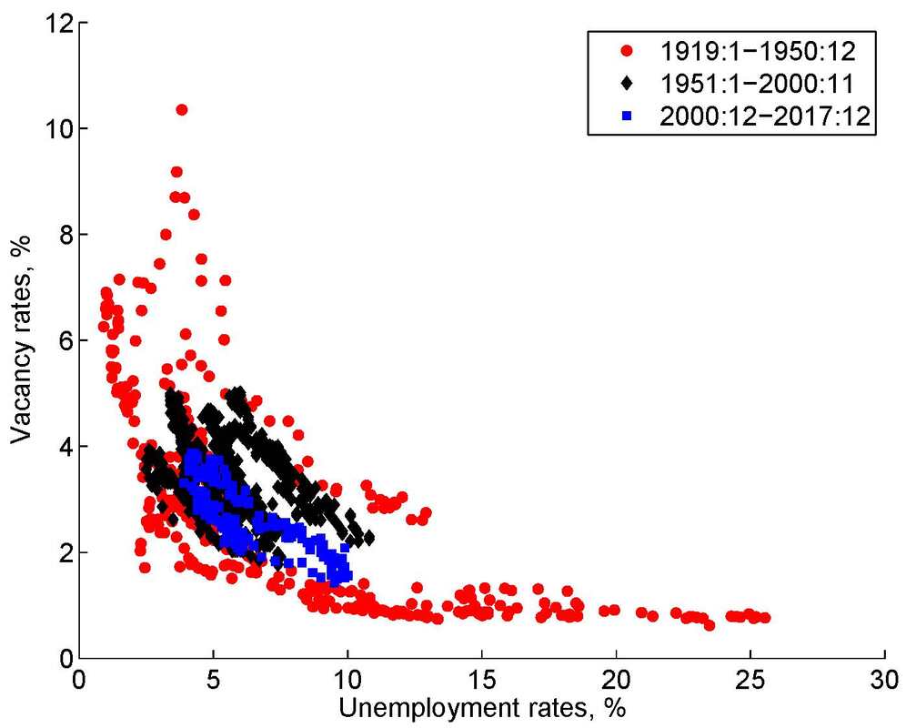 Theoretically, we show that a search model of equilibrium unemployment, when calibrated to the mean and volatility of the postwar unemployment rates, implies empirically plausible persistence and unconditional probability of unemployment crises (states with the unemployment rates above 15%).
We also implement a Cole-Ohanion style accounting exercise for the Great Depression, but within the search framework. With a measured negative labor productivity shock that amounts to a magnitude of 3.4 unconditional standard deviations in the postwar sample, the model predicts a 35.8% drop in output from 1929 to 1933 and a high unemployment rate of 32.9% in June 1933. Both are empirically plausible. We also demonstrate the impact of detrending on the accounting exercise, a point that has not been emphasized in the prior literature. All in all, we suggest that a unified search model with the same parameters is a good start to understanding labor market dynamics in both the pre- and post-war samples simultaneously. |
Lu Zhang
An aspiring process metaphysician Archives
September 2025
Categories |
 RSS Feed